Space/Scale/Time dynamics of two-phase flows

Contact:

Context and Motivation
Two-point statistical equations
Integral geometric measures
Investigated flows

Context

Turbulent two-phase flows are multi-scale and multi-dimensional phenomena, i.e. which depends on:

– the region within the flow,
– the scales of the involved liquid structures
– the fluid/flow physical parameters.

When breaking-up, these liquid structures have complex

– geometry (surface area, curvatures),
– morphology (sphericity, ligamentarity)
– topology (connectedness)
– dynamics (singularity at finite time)

Motivation

Tackling the complexity and the multi-scale facets of liquid atomization requires elaborating a new theory:

– which draws explicit links with the geometry, morphology and topology of the liquid-gas interface,
– which allows scrutinizing the transport of liquid in both scale- and flow-position-space
– which allows some degree of predictibility and regularity to be recovered (in the statistical sense).

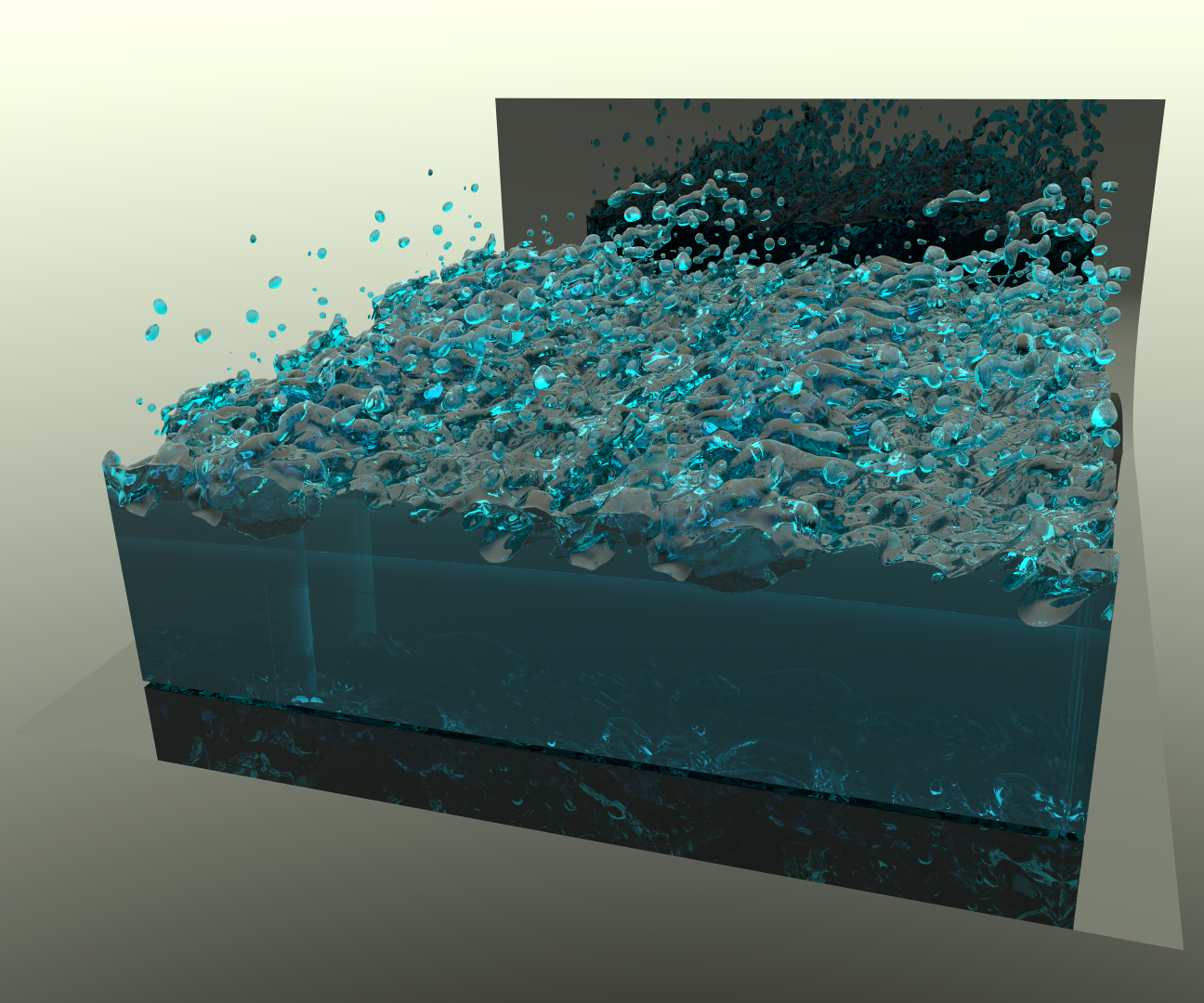
Realistic rendering of a liquid-gas shear flow simulated by the ARCHER code

Schematic representation of the phase indicator field $\phi$ . Gray zones represent the liquid phase ( $\phi=1$ ), white zones the gas phase ( $\phi=0$ ). The two points $\boldsymbol{x^+}$ and $\boldsymbol{x^-}$ together with the mid-point $\boldsymbol{X}$ and the separation vector $\boldsymbol{r}$ are also sketched.

Two-point statistical equations

We proposed using the machinery of two-point statistical equations which originates from the single-phase turbulence community which is adapted here to a relevant scalar in two-phase flows: the phase indicator function $\phi$ . This field variable is simply defined as:

(1) $\begin{equation*} \phi(\boldsymbol{x}) = \left\{ \begin{array}{ll} 1 \textrm{~~~in the liquid phase} \\ 0 \textrm{~~~in the gas phase} \end{array} \right. \end{equation*}$

The transport equation for $\phi$ reads

(2) $\begin{equation*} \partial_t \phi + \boldsymbol{u} \cdot \boldsymbol{\nabla_x} \phi =0 \end{equation*}$

Writing Eq. (2) at two points $\boldsymbol{x^+}$ and $\boldsymbol{x^-}$ , arbitrarily separated by a distance $\boldsymbol{r}$ , one obtains after some manipulations:

(3) $\begin{equation*} \partial_t \langle (\delta \phi)^2 \rangle + \boldsymbol{\nabla_r} \cdot \boldsymbol{\Phi_r} + \boldsymbol{\nabla_X} \cdot \boldsymbol{\Phi_X} =0 \end{equation*}$

In Eq. (3),

$\delta \phi =\phi (\boldsymbol{x^+}) - \phi (\boldsymbol{x^-})~~~~$ is the increment (the difference) of $\phi$ between the two points,
$\langle (\delta \phi)^2 \rangle$ is called the second-order structure function of $\phi$ ,
$\boldsymbol{\Phi_r} = \langle (\delta \boldsymbol{u})(\delta \phi)^2 \rangle$ is the flux of $\phi$ in scale space $\boldsymbol{r}$ . It is generally referred to as the cascade process from one scale to the other.
$\boldsymbol{\Phi_X}\langle (\sigma \boldsymbol{u})(\delta \phi)^2 \rangle$ is the flux of $\phi$ in flow-position space $\boldsymbol{X}$ , i.e. from one position in the flow to the other.
The brackets denote average (to be specified)

Integral geometric measures

The litterature of porous media makes extensive usage of two-point statistics of the phase indicator. Some analytical results allows $\langle (\delta \phi)^2 \rangle$ to be related to some geometrical properties of the liquid-gas interface. In particular, at small scales, the expansion of the second-order increments up to third order writes:

(4) $\begin{equation*} \langle (\delta \phi)^2\rangle_{\Omega} = \frac{\Sigma r}{2} \left[1 - \frac{r^2}{8} \left( \langle H^2\rangle_S - \frac{\langle G\rangle_S}{3} \right) \right] \end{equation*}$

In Eq. (4)

$\Sigma$ is the surface density of the liquid-gas interface
$\langle H^2\rangle_S$ is the area weighted averaged (squared) mean curvature
$\langle G\rangle_S$ is the area weighted Gaussian curvature
$\langle \bullet \rangle_\Omega$ is the angular average (over all orientations of the separation vector $\boldsymbol{r}$ )

Hence, the limit at small scales of Eq. (3) naturally degenerates to the transport equation for the surface density which reads

(5) $\begin{equation*} \partial_t \Sigma + \boldsymbol{u} \cdot \boldsymbol{\nabla_x} \Sigma = \mathbb{K} \Sigma \end{equation*}$

where $\mathbb{K}$ is the stretch rate. At larger scales, $\langle (\delta \phi)^2\rangle$ is expected to provide insights into the tortuousness of the interface.

Simulation of the Plateau-Rayleigh instability using the ARCHER code. The surface is coloured by the local mean curvature $H$ .

(top) Simulation of homogeneous decaying liquid-gaz turbulence. (bottom) Simulation of liquid-gas shear flow. Both were carried out using the ARCHER code

Investigated flows

Homogeneous decaying liquid-gas turbulence

The framework has been first tested in homogeneous decaying liquid-gas turbulence. Homogeneity implies that the gradient w.r.t $\boldsymbol{X}$ vanishes, thereby reducing the problem to the analysis of the scale/time evolution of the system (a 4D problem which depends on $\boldsymbol{r}$ and $t$ ).

Highlights:

– There exists a characteristic length-scale based on the surface density and liquid volume that allows characterizing the scale evolution of $\langle (\delta \phi)^2\rangle$
– The stretch rate $\mathbb{K}$ drives the cascade process of the liquid phase and hence plays the same role as the scalar dissipation rate for diffusive scalars.

Results have been published in Journal of Fluid Mechanics:

F. Thiesset, B. Duret, T. Ménard, C. Dumouchel, J. Reveillon, F.-X. Demoulin. 2020. Liquid transport in scale space. J. Fluid Mech. 886, A4.

Liquid-gas sheared turbulence

We then extended the analysis to a temporally evolving liquid-gas shear layer. In this situation, homogeneity holds only along two directions and one has to resort to the 5D version of the scale/space/time budget (3 dimensions for $\boldsymbol{r}$ , 1 inhomogeneity direction, 1 dimension of time).

Highlights:

– The complexity of liquid transport in the combined space of scales and flow positions is exemplified.
– Some range of scales and flow positions comply with a direct transfer of ‘energy’ (from large to small scales), some others with an inverse cascade.

Results have been presented at the ILASS conference:

F. Thiesset, C. Dumouchel. T. Ménard, 2021. Space-scale-time dynamics of liquid–gas shear flow. J. Fluid Mech 912, A39

F. Thiesset, T. Ménard, C. Dumouchel. 2019. A New Theoretical Framework for Characterizing the Transport of Liquid in Turbulent Two-Phase Flows. ILASS-Europe, Paris, France.